A linear regression model intrinsically interpretable. It is straightforward to calculate the marginal contribution of its features.
“The aim of science is to seek the simplest explanations of complex facts”
― Alfred North Whitehead
A linear regression model is intrinsically interpretable. Its mechanics are transparent and it is fairly straightforward to calculate the marginal contributions of its features.
A black-box model is ideal for modelling complex relationships. It has a clear input and output. However, its inner workings are difficult to investigate.

This blog is focused on calculating the marginal contributions of a linear regression model (Shapley values).
Marginal contribution explained
The marginal contribution of a data point Xi is defined as the deviation of the prediction for a certain data point from the average population, due to the feature.
A linear regression model is explained by using its statistical components. Assume a linear regression:

The marginal contribution of X1 is calculated as:


Explainability in practice
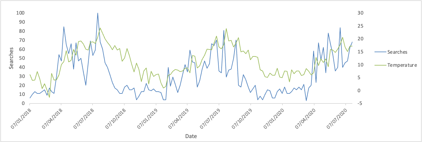
The modelling exercise below will shed some light on the contribution of temperature and holidays on the ice-cream searches using a linear regression model. The data is based on Google Trends data of people searching for the word “softijs” (Dutch word for ice-cream) joined to the temperature and school holidays data.
7 Jan 2018 5 6.1 1
14 Jan 2018 14 3.9 0
21 Jan 2018 10 4.1 0
28 Jan 2018 10 7.4 0
4 Feb 2018 15 4.6 0
... ... ... ...
28 June 2020 51 20.6 0
5 July 2020 52 16.8 1
12 July 2020 44 15 1
19 July 2020 48 17.1 1
26 July 2020 49 17.2 1
The searches dataset shows a clear pattern. Ice-cream searches are more popular during the summer months and less popular during the winter and autumn.
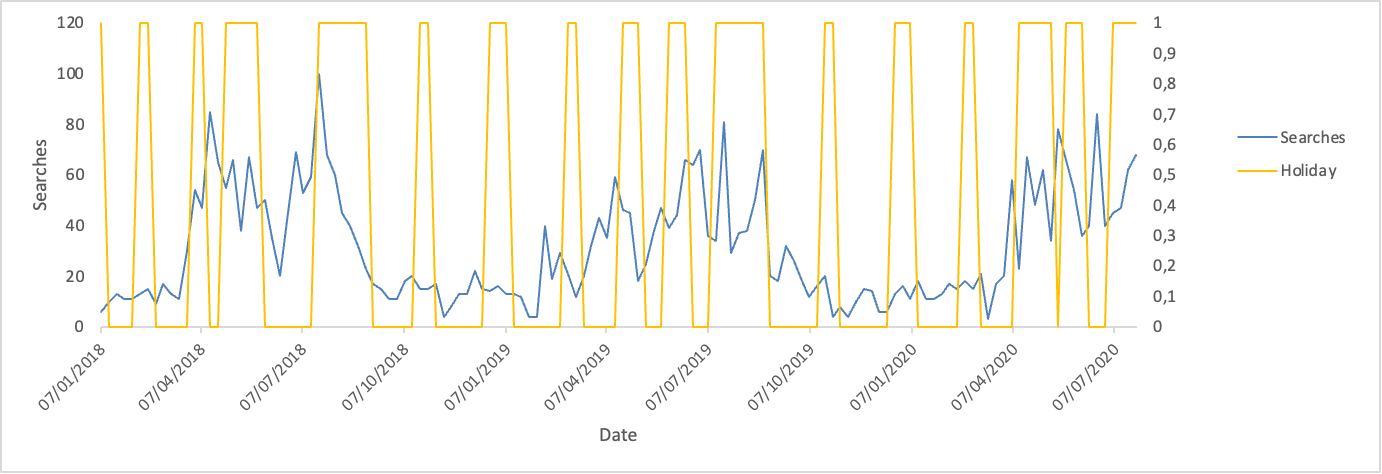
Holidays coincide with a few of the spikes in the searches for ice-cream. However, they do not seem to contribute largely to the ice-cream searches.
For the modelling part, first a linear regression model is applied to the dataset.
from sklearn.linear_model import LinearRegression
pdf_model = pdf.copy()
pdf_model = pdf_model.set_index(date_col)
y = pdf_model[target_col]
x_test = X[-1:]
y_train = y[:-1]
y_test = y[-1:]
fitted_model = model.fit(x_train, y_train)
return fitted_model, x_train, x_test, y_train
Next, the marginal contribution of each feature is calculated:
coef = model.coef_
local_explainer_linear = (X - X.mean(0)) * coef
return local_explainer_linear
print(local_explainer_linear)
Here are the results:
7 Jan 2018 -10.6 3.4
14 Jan 2018 -15.3 -2.4
21 Jan 2018 -14.9 -2.4
28 Jan 2018 -8.1 -2.4
24 Jan 2018 -13.9 -2.4
... ... ...
21 June 2020 13.6 -2.4
28 June 2020 19.5 -2.4
5 July 2020 11.7 3.4
12 July 2020 7.9 3.4
19 July 2020 12.4 3.4
The marginal contribution of temperature in the 28th of June 2020 is +19.5. This means that the estimated number of searches due to higher temperature is 19.5% more than average. The average temperature for this month is 16.5°C. The positive impact makes sense, since ice-cream is a popular treat during the summer months when the temperature is high.
Looking at the results for a colder month, the marginal contribution of temperature in January 2018 is negative, when the average temperature is 5.4°C. People eat less ice-cream during the coldest months of the year.
During Christmas and summer school holidays, the marginal contribution of holidays is positive. In festive dinners a dessert is often served, ice-cream being one of the options. Also, children buy more ice-cream when they are on holiday.
Conclusion
Explaining a linear regression model is a straightforward process which is easily implemented. Calculating the marginal contributions gives a clear view of the mechanics of the model. This allows a data scientist to validate the output, explain the predictions to stakeholders with more confidence and tune the model based on the findings.
Sources
[1] “Comparing black-box vs. white-box modeling” by Tamanna: https://medium.com/@tam.tamanna18/comparing-black-box-vs-white-box-modeling-bd01575b7670#:~:text=Even%20in%20less%20complex%20scenarios,a%20churn%20detection%20use%20case.