24 februari

Time-series as a signal: Fast Fourier transform to decompose seasonality

Frida Karvouni
Auteur

The easiest way to model seasonality is by using seasonal dummies. A more scientific method is to apply Fast Fourier Transform (FFT).

Definition of seasonality

Seasonality is defined as a repetitive pattern over a particular time period. It holds information on repeating patterns of customers’ shopping behaviour and product availability. Therefore, it is an important feature to capture within a time-series machine learning model.

Ways to model seasonality

The simplest way to model seasonality is to add time-related features. Examples of such seasonality indicators are:

Quarter of the year
Day of the week
ISO week of the year
Month of the year
Warm/ cold weather indicator: one feature describing reasonably warm or cold months (Relatively warm months are the ones in quarters 2 and 3 and relatively cold months are in quarters 1 and 4)

These features have the benefit of being very easy to implement. The downside is that they undesirably capture the effect of recurrent business decisions.

Fast Fourier Transform (FFT)

A more scientific method of modelling seasonality is to create a Fourier term. The Fast Fourier Transform (FFT) method creates a sinusoid (Fourier term) which is repeated over a specified period of time.

Basic components of a Fourier term

A Fourier term is composed from the following components:

Amplitude: the magnitude of the peak value
Period: the amount of time required to complete one full cycle

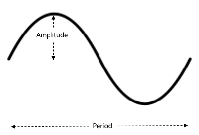
Frequency: the number of observations measured before the seasonal pattern repeats

Practical example

A practical example would make the theory easier to understand. The Google trends data for the searches of the keyword “meloen” (Dutch word for “melon” was used in this example. Here is a plot of the time series for a time period of four years.

It can be easily seen in the plot above, that searches for melon start to increase somewhere in June and peak in July for all years. This would give an indication that there is seasonality around summer.

The hypothesis may be tested with the following seasonality test:

import pandas as pd
from scipy.stats import friedmanchisquare

def seasonality_test(input_data: pd.DataFrame, label_field: str) -> bool:
input_data["year"] = pd.DatetimeIndex(input_data["date"]).year
input_data["month"] = pd.DatetimeIndex(input_data["date"]).month

transformations = {label_field: "mean"}

input_data = input_data.groupby(["year", "month"]).agg(transformations)
input_data.reset_index(inplace=True)

    min_year = input_data[input_data["month"] == 1]["year"].min()
    max_year = input_data[input_data["month"] == 12]["year"].max()
    input_data = (input_data[(input_data["year"] >= min_year) &
                 (input_data["year"] <= max_year)])

year_values = [year for year in input_data["year"].unique()]

number_of_years = len(year_values)

input_data = input_data.pivot(index="month", columns="year",
values=label_field)

    stat, p = friedmanchisquare(
        input_data[year_values[number_of_years - 3]],
        input_data[year_values[number_of_years - 2]],
        input_data[year_values[number_of_years - 1]])

print(f"Statistics = {stat}, p = {p}")

    alpha = 0.01
    if p > alpha:
        print("Same distributions (fail to reject H0)")
        season = True
    else:
        print("Different distributions (reject H0)")
        season = False
    return season

season = seasonality_test(input_data=pdf, label_field="searches")
print(f"Seasonality is: {season}")

>> Statistics = 0.383, p = 0.826
>> Same distributions (fail to reject H0)
>> Seasonality is True

The seasonality test indicates that it failed to reject null hypothesis H0, thus seasonality is present in the dataset.

This is indeed confirmed by searching for the crop season for melon in the Netherlands, which is three months: namely June, July and August. This would be the time when a lot of people living in the Netherlands would search where to buy melons from or on information on how to grow melons.

The FFT can be used to model the seasonality indicated by the test above.

import math
from cmath import phase
import numpy as np
import pandas as pd
from scipy import fft
from scipy import signal as sig
from sklearn.linear_model import LinearRegression
import matplotlib.pyplot as plt
import seaborn as sns

def add_trend_term(pdf):
pdf["trend"] = pdf.apply(lambda row: row.name + 1, axis=1)
return pdf

def add_fourier_seasonality_term(pdf, column_name, period_min, period_max):
    # Performs fourier transformation
    fft_output = fft.fft(pdf[column_name].to_numpy())
    amplitude = np.abs(fft_output)
    freq = fft.fftfreq(len(pdf[column_name].to_numpy()))

    mask = freq >= 0
    freq = freq[mask]
    amplitude = amplitude[mask]

    # determine peaks
    peaks = sig.find_peaks(amplitude[freq >= 0])[0]
    peak_freq = freq[peaks]
    peak_amplitude = amplitude[peaks]

    # Create dataframe containing necessary parameters
    fourier_output = pd.DataFrame()
    fourier_output["index"] = peaks
    fourier_output["freq"] = peak_freq
    fourier_output["amplitude"] = peak_amplitude
    fourier_output["period"] = 1 / peak_freq
    fourier_output["fft"] = fft_output[peaks]
    fourier_output["amplitude"] = fourier_output.fft.apply(lambda z: np.abs(z))
    fourier_output["phase"] = fourier_output.fft.apply(lambda z: phase(z))

N = len(pdf.index)
fourier_output["amplitude"] = fourier_output["amplitude"] / N

    fourier_output = fourier_output.sort_values("amplitude", ascending=False)
    fourier_output = fourier_output[fourier_output["period"] >= period_min]
    fourier_output = fourier_output[fourier_output["period"] <= period_max]

    # Turn our dataframe into a dictionary for easy lookup
    fourier_output_dict = fourier_output.to_dict("index")
    pdf_temp = pdf[["trend"]]

lst_periods = fourier_output["period"].to_list()
lst_periods = [int(round(val, 0)) for val in lst_periods]

    for key in fourier_output_dict.keys():
        a = fourier_output_dict[key]["amplitude"]
        w = 2 * math.pi * fourier_output_dict[key]["freq"]
        p = fourier_output_dict[key]["phase"]
        pdf_temp[key] = pdf_temp["trend"].apply(
                        lambda t: a * math.cos(w * t + p))

    pdf_temp["FT_All"] = 0
    for column in list(fourier_output.index):
        pdf_temp["FT_All"] = pdf_temp["FT_All"] + pdf_temp[column]

pdf["seasonality"] = pdf_temp["FT_All"].astype(float)
pdf["seasonality"] = pdf["seasonality"].round(4)

    predictors = ["trend", "seasonality"]
    X = pdf[predictors]
    y = pdf["searches"]

X_predict = pdf[predictors]

    # Initialise and fit model
    lm = LinearRegression()
    model = lm.fit(X, y)

    # Forecast baseline for entire dataset
    pdf["baseline"] = model.predict(X_predict)
    pdf["baseline"] = pdf["baseline"].round(4)
    return (fourier_output, pdf)

def create_plots(pdf, period_min, period_max):
pdf = pdf.reset_index()
pdf = add_trend_term(pdf=pdf)

    (fourier_output, pdf) = add_fourier_seasonality_term(
        pdf,
        column_name="searches",
        period_min=period_min,
        period_max=period_max
    )

pdf["date"] = pd.to_datetime(pdf["date"], format="%Y-%m-%d")
pdf = pdf.set_index("date")

    fig, axs = plt.subplots(ncols=1, figsize=(30, 5))
    sns.lineplot(data=pdf, x="date", y="searches",
                 label="searches", color="grey")

    sns.lineplot(x="date", y="baseline", data=pdf, ax=axs,
                 label="baseline", color="black")
    axs.legend()
    plt.show()

By adjusting the min_period and max_period parameters, a sinusoid is applied on a level specified based on the underlying data.

Experiment #1: Create a sinusoid on a weekly level

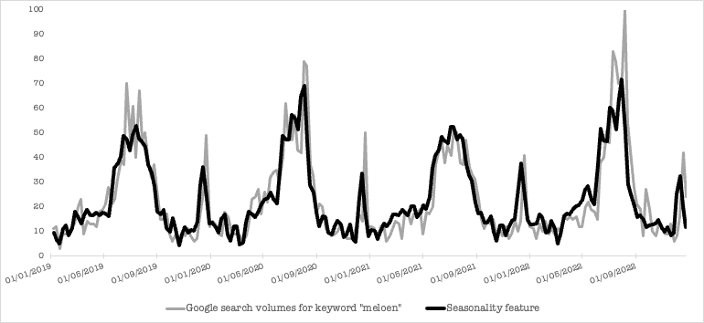
create_plots(pdf=pdf, period_min=3, period_max=52)

The first experiment is not satisfactory as it overfits on the underlying data and captures noise as seasonality. Melon is used for some Christmas dishes so the searches peak in December. This peak is considered noise and should not be modelled as seasonality.

Experiment #2: Create a sinusoid on a yearly level

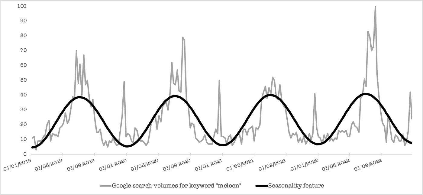
create_plots(pdf=pdf, period_min=52, period_max=62)

The Fourier term in the second experiment captures the yearly seasonality for melon. The Fourier term may be used as a feature when building a model to capture seasonality.

Conclusions

Seasonality is an important aspect of a time series dataset. There is an easy way to model it by using seasonal dummies. A more scientific method is to apply FFT to model seasonality for a specified time period.